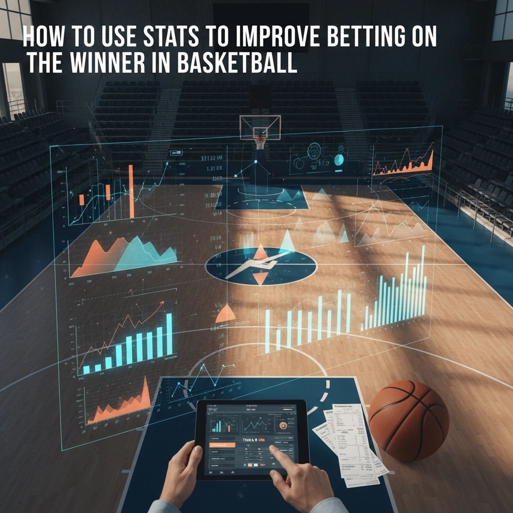
Why reading the right basketball stats changes how you pick the winner
You probably know that betting on the winner (moneyline) looks simple: one team wins, you get paid. But bookmakers set lines using a mix of team form, injuries, public money and advanced metrics. If you only follow headlines or gut feeling, you miss the structural edge that numbers provide. By focusing on the right statistics you can quickly spot value bets where the market misprices a team’s true chances.
Stats force you to separate noise from signal. For example, a team on a long win streak may be overvalued if that streak came against weak defenses or in slow-paced games. When you compare objective metrics — pace, efficiency, turnover rates — you get a clearer picture of whether a team’s recent wins are sustainable and whether the available odds reflect that reality.
Which statistics matter most when betting on the winner and why
Not all stats are equally useful for moneyline betting. You want metrics that estimate scoring ability and defensive resistance while adjusting for pace and opponent quality. Below are high-impact statistics and how you should interpret them:
- Net Rating (Offensive Rating − Defensive Rating): This is the best single indicator of team strength. A positive net rating means a team scores more points per 100 possessions than it allows. Use net rating to compare teams directly, especially after adjusting for home/away splits.
- Tempo / Pace: Points per 100 possessions matter more than raw points. Teams with high pace create more possessions and variance — which affects underdog value in moneyline bets. A slow, efficient team can be favored in close games.
- Field Goal and 3P% Adjusted for Quality of Opposition: Shooting efficiency against league-average defenses is more telling than raw percentage. Look at effective field goal percentage (eFG%) and opponent-adjusted splits.
- Turnover Rate and Opponent Turnover Rate: Teams that protect the ball and force turnovers change possession value. A mismatch here often flips expected outcomes, especially in close contests.
- Rebounding Rates (Offensive/Defensive): Rebounding impacts second-chance points and possession control. A team that consistently dominates the glass can neutralize superior perimeter shooting.
- Injury and Lineup-adjusted Stats: Many stats change drastically when a key player is out. Look at on/off splits and lineup data to see how the team’s net rating shifts with or without starters.
Once you’ve identified the relevant stats, your next step is to synthesize them into an actionable view. You do this by comparing team profiles (pace, net rating, shooting, turnovers, rebounding) and adjusting for contextual factors like travel, rest, and matchup quirks (e.g., a poor perimeter defense facing a hot-shooting opponent). Simple comparative charts or a short checklist help you rank which team has the structural advantage.
In the next section, you’ll learn a straightforward process to combine these metrics into a quick pre-game model and how to adjust it live during the game to find profitable moneyline opportunities.
Build a simple pre-game model you can run in five minutes
Start with the handful of numbers that matter and put them into a consistent framework. Here’s a compact process you can do in a spreadsheet or on paper before every game:
1. Gather core inputs
– Team Net Ratings (use home/away splits if available).
– Team Pace (possessions per 48 minutes or per game).
– Relevant lineup/on‑off adjustments for any injuries or confirmed absences.
– Bookmaker moneyline (convert to implied probability).
2. Adjust for context
– Add a home-court bump (commonly 2.5–3.0 points in the NBA; use league-specific values).
– Subtract for travel/rest penalties (e.g., road team on second night of back‑to‑back: −1 to −2 points).
– Swap in lineup-adjusted net ratings when a key player is out.
3. Convert net rating difference into an expected point margin
– Net rating is points per 100 possessions. Find the matchup’s expected possessions (use the average of both teams’ pace).
– Expected margin = NetRatingDiff × (ExpectedPossessions / 100).
– Example: Team A net rating − Team B net rating = +5; expected possessions = 98 → expected margin ≈ 5 × 0.98 = +4.9 points for Team A.
4. Turn margin into a win probability
– Use a normal approximation: WinProb = CDF( expected_margin / SD ).
– A practical SD for single-game point differential is around 12–13 points. Using 13: z = margin / 13; WinProb = normal CDF(z).
– Example (from above): margin 4.9 → z ≈ 0.377 → WinProb ≈ 65%.
5. Compare to the market and act
– Convert the moneyline to implied probability. For a negative favorite: implied = |ML| / (|ML|+100). For a positive underdog: implied = 100 / (ML+100).
– If your model’s win probability exceeds the implied probability by your edge threshold (commonly 3%+ to account for vig and model error), that’s a potential value bet.
– Size bets using a conservative staking rule — flat units or Kelly with a cap — not full bankroll swings.
This gives you a repeatable, defensible pre-game edge-finder that’s fast and transparent.
Adjusting the model live: what to watch and when to act
Pre-game models are your baseline; live betting rewards quick, disciplined updates when the game narrative or inputs change. Use these signals and a simple recalculation to find in-game value:
– Immediate triggers: confirmed injury/benching, ejection, or a star in foul trouble. Switch to lineup-adjusted net ratings as soon as the change is official.
– Momentum triggers: sustained runs caused by turnovers, offensive rebounding surges, or a sudden pace shift. If one team forces turnovers at a much higher rate than expected, estimate the possession swing and adjust expected margin.
– Shooting variance: short-term hot/cold streaks happen. Don’t overreact to a couple of makes/misses unless they coincide with a structural change (e.g., defender out, new matchup).
A practical live update method
1. Calculate remaining possessions (roughly: (time left in minutes / 48) × expected possessions).
2. Expected additional margin = NetRatingDiff × (RemainingPossessions / 100).
3. Projected final margin = CurrentScoreDiff + Expected additional margin.
4. Adjust SD for fewer possessions: use SD × sqrt(RemainingPossessions / 100) to reflect reduced variance late in games.
5. Recompute win probability with the adjusted SD and compare to live moneyline implied probability.
Example: tied game, 12 minutes left (~24 possessions), net rating diff implies +6 over 100 possessions. Remaining expected margin = 6 × 24/100 = +1.44 → projected final margin ≈ +1.44. Adjust SD: 13 × sqrt(24/100) ≈ 6.4 → z = 1.44/6.4 ≈ 0.225 → WinProb ≈ 59%. If the live moneyline implies 50–52%, that’s a live value opportunity.
Rules of thumb for action
– Require a clear edge (3%+ in pre-game; 5%+ when markets are more efficient in-play).
– Bet quickly on confirmed lineup/injury news — markets lag most on subtle rotation changes.
– Reduce stake as uncertainty rises (late-game variance, low liquidity) and avoid overbetting on “feel” momentum without a structural change.
Using these simple calculations keeps your live bets systematic and lets you exploit slow market reactions without chasing noise.
Putting it into practice
Start small and iterate. Run the five-minute pre-game process for a handful of games each week, track every bet (model probability, market implied probability, stake, outcome), and review where your model is systematically off. Backtest adjustments before using them with real money and keep a strict staking plan — conservative Kelly caps or flat units work well while you validate performance.
- Keep a simple log: date, teams, model edge, market price, stake, result. Review monthly.
- Calibrate your SD and home-court/rest adjustments from your own sample rather than relying solely on generic values.
- Use reliable data sources for inputs (for example, Basketball-Reference) and automate what you can to avoid manual errors.
Approach this as an iterative engineering problem: small, repeatable improvements compound. Respect variance, protect your bankroll, and keep emotion out of sizing decisions. Over time the discipline of a simple statistical process will separate transient luck from genuine edges.
Frequently Asked Questions
How should I pick the SD value when converting margin to win probability?
Use a league- or sample-specific SD if possible. The article uses ~13 points for a typical single-game SD in the NBA as a practical starting point. Better is to calculate the standard deviation of final point differentials from recent seasons or from your own tracked sample and update it periodically.
What stake sizing method is safest while validating a new model?
Start with flat units (a fixed small percentage of bankroll) or a fractional Kelly approach with a cap (for example, half-Kelly with a maximum of 2–3% of bankroll). These methods limit downside while allowing you to learn from real-world results without overexposure to variance or model miscalibration.
Can I apply this pre-game and live-adjust framework to college basketball or other leagues?
Yes. The same framework applies, but you must adjust core inputs: home-court advantage, possessions per game (pace), typical SD, and injury/rotation volatility differ across leagues. Re-estimate those parameters from league-specific data before using the model live.